Music Source Separation with TPU at Deep Learning Camp Jeju 2018
deep-learningBy Olga Slizovskaia and Leo Kim
What brought us all together at Jeju
We were very fortunate to have been part of the Deep Learning Camp Jeju 2018, organized by Tensorflow Korea for one whole month of July. The camp was held in Jeju, a beautiful island located just south of the Korean peninsula, where 24 lucky applicants from all over the world gathered to work on their research projects. We had never met prior to this camp, but our mentor Terry Um was quick to find out that we shared similar interests, and paired us up to work as a team. We quickly got along through our mutual enthusiasm for music. After spending some time bouncing ideas back and forth, we decided to work on music source separation using deep learning.
First group trip to Sangumburi crater in Jeju island
In this article, we give an introduction to music source separation and briefly discuss possible approaches. Then we explain which architecture and datasets we used in our project and what modifications we made. We dedicate the next part of the post to a practical step-by-step guide for reproducing our experiments and running a model on TPU. Finally, we discuss the results and our experience and impression of the camp.
What is music source separation?
The goal of music source separation is to extract the mixture of audio sources that have been recorded in mono channel into their individually separated source tracks. Common application areas include vocal isolation from accompaniments, or extracting individual instrument sources from multi-instrument recordings such as an orchestral track for post-production, remixing and MIR (music information retrieval) which can be further applied to music recommendation systems and more. Undoubtedly, this is a very challenging problem to solve and many attempts have been made to estimate the source signals as close as possible from the observation of the mixture signals. Here is a short video clip that demonstrates the goal we would like to achieve: https://youtu.be/dqLyjzvXepA
There are many challenging aspects of audio source separation. Most importantly, accurate separation with minimal distortion is desired. Supplementary information such as the number of sources present in the mix, musical notes in the form of MIDI or sheet music can be helpful but not widely available in most cases. However, we noticed an increasing trend in video availability on the web, many including recordings of musical instruments. In the later sections, we will describe how we took this to our advantage in assisting source separation.
What methods are there for music source separation?
Traditionally, people have attempted to solve audio source separation through matrix-factorization algorithms. Independent Component Analysis (ICA) is one of the common techniques used for blind source separation. Under the assumption that the different physical processes create unrelated signals, ICA can be applied to extract individual signals from mixtures by leveraging statistical independence between signals. Principal Component Analysis (PCA) is very similar to ICA because it also projects data into a new set of axes based on a statistical criterion. However, instead of measuring the non-Gaussianity of signal like in the ICA, PCA recursively chooses axes that maximize variance to separate the signals.
Another popular technique used is the Non-negative Matrix Factorization (NMF). NMF is an algorithm that factorizes a non-negative matrix X, into a product of two non-negative matrices W and H by iteratively minimizing the distance between the X and the product of WH. The input matrix X is the spectrogram obtained from the Fast Fourier Transform of the audio source, W is the frequency response of the source at each time frame, and H is the activation gain of frequency at each time frame. The divergence between X and WH is minimized with multiplicative updates until a pre-decided number of epochs or until the divergence falls below a certain threshold.
With the recent achievements in machine learning, researchers have started to adopt a deep neural network paradigm to source separation domain. CNNs have been proven to be successful in image processing, so commonly raw audio data is converted to 2-D spectrogram images. Then the image data is fed to a convolutional autoencoder which generates set of masks that can be used to recover sound sources using inverse Short Time Fourier Transform.
What is our approach and how is it different from the traditional ways?
For our project, we wanted to continue researching deep learning methods to solve the blind source separation problem. Furthermore, we wanted to focus on improving the results by experimenting with less conventional approaches. Primarily, we wanted to work directly with raw waveforms as opposed to time-frequency image representation. Secondly, we wanted to enhance our results through conditioning with visual input from the video data.
Model architecture
We began our project by first adapting the Wave-U-Net architecture which can handle end-to-end audio source separation using raw audio bits in the time domain. We thought this was a rather a novel approach compared to the conventional source separation methodologies which often involves transforming the data into the frequency domain and performing analysis on the spectrograms. By using models with less complexity, we hoped to achieve a more natural way of recovering source separation.
Wave-U-Net
Wave-U-Net model is an adaptation of the U-Net. But instead of doing a 2D convolution, Wave-U-Net performs a series of 1-D convolution downsampling and upsampling with skip connections on raw WAV files. The input to this network is a single channel audio mix, and the desired output is the separated K channels of individual audio sources, where K is the number of sources present in the audio mix. One thing that is really neat about the Wave-U-Net is that it avoids implicit zero paddings in the downsampling layers, and it performs linear interpolation as opposed to de-convolution. This means that our dimension size is not preserved, and our output results will actually become a lot shorter compared to our input. However, by doing this we can preserve better temporal continuity and avoid audio artifacts in our results. Here is a demo from the results we got from training the original Wave-U-Net https://youtu.be/mGfhgLt1Ds4
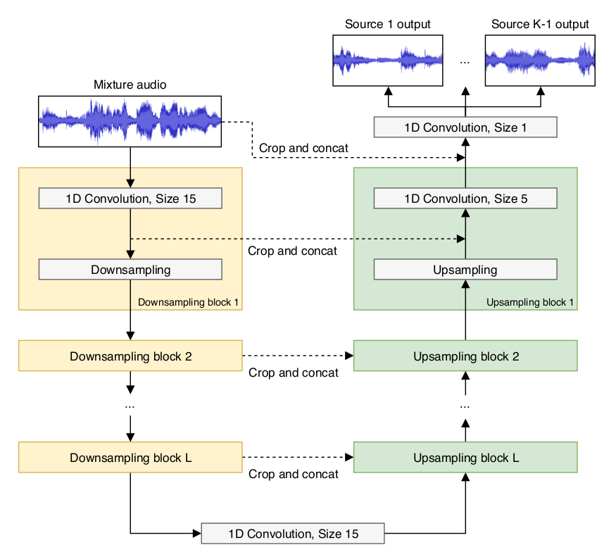
Original Wave-U-Net model with K sources and L layers
Expanded Wave-U-Net
The challenge with the original Wave-U-Net model is that it can only support a predefined number of input sources, limiting its application to only a specific group of music that it is trained on. We wanted to build a flexible model that can support a “dynamic” number of input sources. This is still not a truly dynamic model since we cannot support an infinite number of sources. However, we can emulate to some degree by fixing the maximum number of sources to a reasonably big number. The sources that are present in the mix can be trained with silent audio as a substitute. Here is the demo of one of the better results we achieved from the expanded Wave-U-Net https://youtu.be/mVqIMXoSDqE
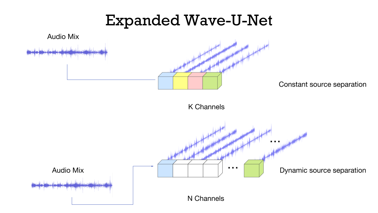
Top: Original Wave-U-Net requires same predefined K number of input sources for every track; Bottom: Expanded Wave-U-Net mimics dynamic separation by training omitted sources with silent waveforms
Conditioned Wave-W-Net
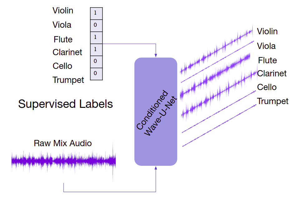
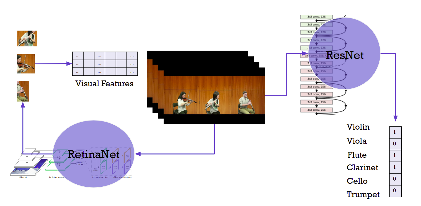
To enhance our results, we proposed a separate vision model that takes inputs from the video frames and apply it for conditioning the audio model. Conditioning is a term used to describe the process of fusing information of different mediums in the context of another medium. The idea is to run object detection on the image frames to identify the instruments which are present in the video. We then condition the audio model to enhance our source separation results with this supplementary information, which can be obtained from manual annotations or learned from the corresponding data from other modalities such as videos or scores.
There are mainly three locations where we could apply conditioning:
- Before downsampling
- At the bottleneck (bottom of Wave-U-Net)
- After upsampling
There are also various conditioning mechanisms that we referenced from this very helpful article titled Feature-wise transformation. The article provides three approaches:
- Concatenation base conditioning
- Conditional biasing (additive bias)
- Conditional scaling (multiplicative bias).
We experimented on multiplicative conditioning using supervised instrument labels at the bottleneck of the Wave-U-Net model.
Original Wave-U-Net model with K sources and L layers
Datasets
Normally, music source separation models are trained in a supervised manner. Therefore, one needs a multi-track dataset that contains the mix and the estimates for the individual sources. Some example datasets that can be used are:
| Dataset | Size (tracks) | Data types | Comments |
|---|---|---|---|
| musdb | 150 | audio | popular songs, 4 sources |
| MedleyDB | 108 | audio | popular songs, many sources |
| Bach10 | 10 | audio, midi | classical music, many sources |
| URMP | 44 | audio, midi, video, scores | classical music, many sources |
The original implementation of the Wave-U-Net model heavily relies on the musdb18 dataset. It contains hardcoded embeddings of data preprocessing and training that is specific to the musdb18 dataset. For our project, we wanted to experiment with both musdb and URMP datasets, and possibly more in the future. To achieve that we modified the data preprocessing step and stored data as TFRecords.
We first created tf.records for both musdb and URMP datasets. Each row in a tf.record contains encoded audio data (a bigger segment for the mix and small segments for sources) and metadata which helps us to properly decode the waveform and do the evaluation later (filename, sample rate, index of the audio segment, number of channels and sources):
example = tf.train.Example(features=tf.train.Features(feature={
  	 'audio/file_basename': _bytes_feature(os.path.basename(filename)),
  	 'audio/sample_rate': _int64_feature(sample_rate),
 	 'audio/sample_idx': _int64_feature(sample_idx),
  	 'audio/num_samples': _int64_feature(num_samples),
  	 'audio/channels': _int64_feature(channels),
  	 'audio/num_sources': _int64_feature(num_sources),
 	 'audio/encoded': _sources_floatlist_feature(data_buffer)}))
Once all tf.record files are created, we can use them for forming a tf.Dataset.
The tf.Dataset is a dataset abstraction that provides easy data shuffling, batching, bufferization and efficient parallel loading, which is crucial for training on TPU.
Typically, it splits a tf.record file into rows and applies a set of processing functions row by row. A standard set may include a parser which parses a single example of the dataset:
keys_to_features = {
   'audio/file_basename': tf.FixedLenFeature([], tf.string, ''),
   'audio/encoded': tf.VarLenFeature(tf.float32),
   'audio/sample_rate': tf.FixedLenFeature([], tf.int64, SAMPLE_RATE),
   'audio/sample_idx': tf.FixedLenFeature([], tf.int64, -1),
   'audio/num_samples': tf.FixedLenFeature([], tf.int64, NUM_SAMPLES),
   'audio/channels': tf.FixedLenFeature([], tf.int64, CHANNELS),
   'audio/num_sources': tf.FixedLenFeature([], tf.int64, NUM_SOURCES)
}
parsed = tf.parse_single_example(value, keys_to_features)
And reshare raw bytes into tensors:
audio_data = tf.sparse_tensor_to_dense(parsed['audio/encoded'], default_value=0)
audio_shape = tf.stack([MIX_WITH_PADDING + NUM_SOURCES*NUM_SAMPLES])
audio_data = tf.reshape(audio_data, audio_shape)
mix, sources = tf.reshape(audio_data[:MIX_WITH_PADDING],
tf.stack([MIX_WITH_PADDING, CHANNELS])),
          tf.reshape(audio_data[MIX_WITH_PADDING:],
tf.stack([NUM_SOURCES, NUM_SAMPLES, CHANNELS]))
labels = tf.sparse_tensor_to_dense(parsed['audio/labels'])
labels = tf.reshape(labels, tf.stack([NUM_SOURCES]))
And cast tensor to bfloat16 (in case you want a bigger batch size)
if self.use_bfloat16:
   mix = tf.cast(mix, tf.bfloat16)
   labels = tf.cast(labels, tf.bfloat16)
   sources = tf.cast(sources, tf.bfloat16)
Training procedure and pipeline
In this project, we took advantage of the Google Cloud Platform for both data storage and computations. The encoded datasets are stored in the buckets as TFRecords, and the tf.Dataset can read the data directly from these buckets.
file_pattern = os.path.join(self.data_dir, 'train-*' if self.mode == 'train' else 'test-*')
dataset = tf.data.Dataset.list_files(file_pattern, shuffle=(self.mode == 'train'))
For training and prediction, we use another high-level TF abstraction such as the tf.Estimator. The tf.Estimator abstracts out distributed training (for multi-GPUs or TPU training), it creates and manages tf.Session and tf.Graph and provides good practices for summary writing.
The computational pipeline looks as follows: we have a VM instance, a client where the code runs, and GPU/TPU as a worker. In the case of using TPU, we have to work with tf.Dataset because input pipeline operations are copied to each remote worker and it can be done only with tf.Dataset. After a pre-defined number of iterations, TPU nodes send metrics and summaries back to the client where the client saves them. We store all checkpoints in a bucket, which is also supported out of the box and provides good performance. Although, It might be a bad idea to store multimedia summaries (images and audio) too often, as it slows down training a lot.
To evaluate the performance of GPU with parallel loading and TPU with tf.Dataset we run a couple of experiments with musdb18 dataset. Below is the performance graph for both runs:
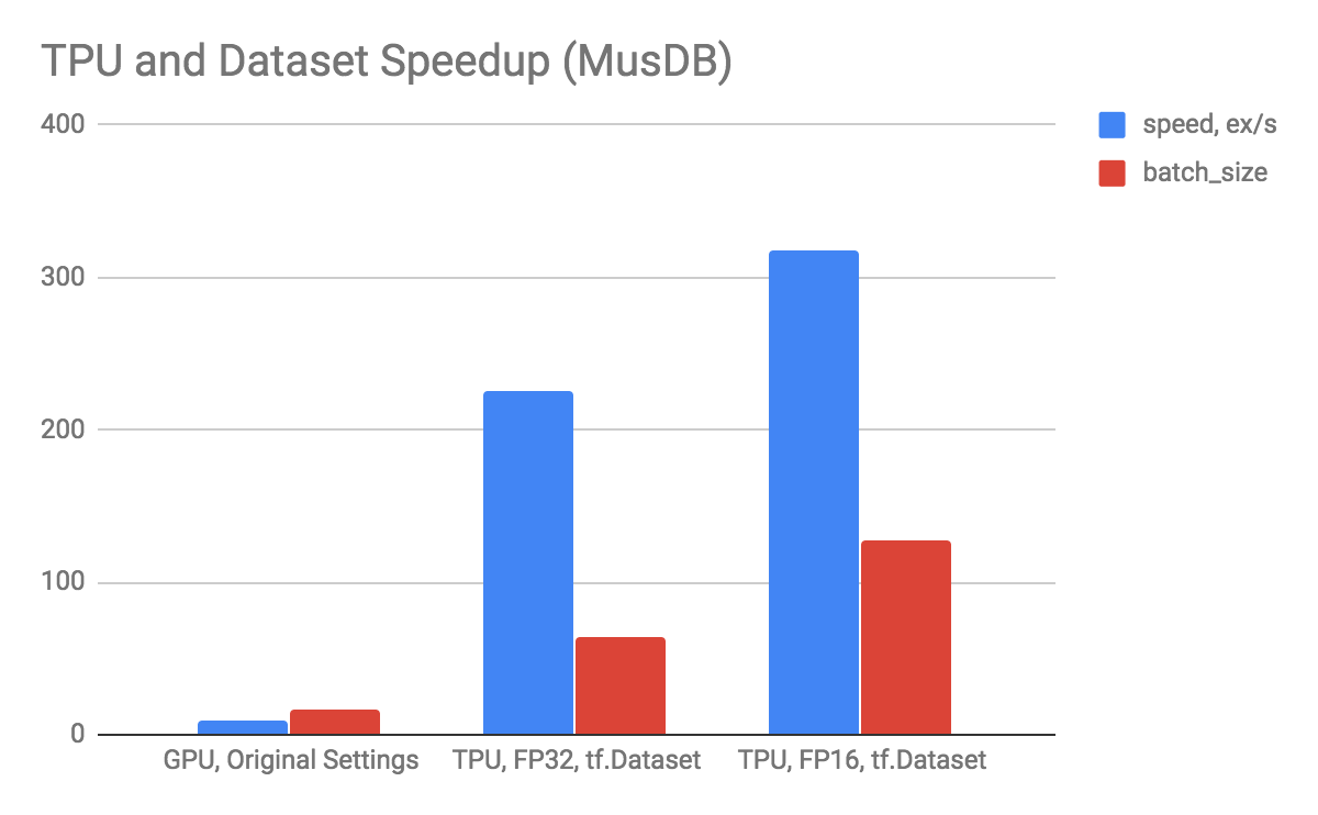
Performance comparison of GPU vs TPU and bfloat16 vs bfloat32
We performed a set of ablation studies and experimented with different learning rates, with and without learning rate exponential decay and label conditioning. Additionally, we used bfloat16 data type in order to enlarge batch size. In the experiments below, we trained a model for 200k epochs on a single TPU unit with Adam optimizer.
Results and demos
There are several standard metrics to evaluate the quality of source separation methods:
- SDR (source to distortion ratio)
- Measures the general performance
- SIR (source to interference ratio)
- Measures suppression of interfering sources
- SAR (source to artifact ratio)
- Measures artifacts generated during the separation process
The metrics are computed as energy ratios and measured in decibels (dB). The higher value of the metric means the lesser effect of the corresponding error (distortion, interference or artifact).
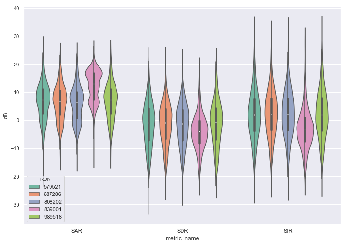
Violin plots of SAR, SDR and SIR segment-wise values for different ablation studies (see the legend below)
Legend: 579521 - Expanded Wave-U-net, lr=1e-05 with exponential decay, MSE loss, dtype=float32 687286 - Expanded Wave-U-net with conditioning, lr=1e-05, SSE loss, dtype=float32 808202 - Expanded Wave-U-net, lr=1e-04, MSE loss, dtype=float32 839001 - Expanded Wave-U-net, lr=1e-05, SSE loss, dtype=bfloat16 989518 - Expanded Wave-U-net, lr=1e-05, MSE loss, dtype=float32
The above metrics were computed on a per segment basis (each segment is about 1-second length) for each non-silent source. The metrics are objective and allow us to evaluate the models quantitatively, but often they don’t reflect perceptual quality. For production applications, it’s recommended to do a listening test to measure the subjective performance of a method. Here we only provide the quantitative evaluation and demos.
What we learned
In the future, we would like to continue investigating better conditioning methods to enhance our separation results while taking training time and costs into considerations. We would also like to come up with a better way to perform a true dynamic source separation where there is no cap on the maximum instruments allowed in the mix. Finally, we would like to adapt our loss functions that can more accurately measure our needs. For this, we would have to first get a better understanding of audio signal processing and music theory.
Possible future implementation
We really enjoyed working with the TensorFlow library and the TPUs. Both of them are excellent researching tools that saved a lot of hours doing the groundwork. We did run into some difficulties while setting up TPU, mainly because the documentation is not yet complete. Especially with writing custom estimators, the official tensorflow website lacked a lot of explanation, and often times we resorted to reading the original code implementations to figure out their functionalities. Debugging with TPU estimators was also not very straightforward due to the way it wraps around Session.run(). Injecting your own debugging messages was very unintuitive. Lastly, we found a few bugs in the TensorBoard. Despite defining the iteration cycle for summary writer, it was being called every iteration, causing a huge bottleneck in our training time. In the end, we had to remove summary writing and train without knowing the intermediate results. Also, the TensorBoard tended to freeze and stop showing updates after some training steps. So to see the newest result, we had to restart the TensorBoard connection, which can take a very long time to load.
Acknowledgements
This project was supported by Deep Learning Camp Jeju 2018 which was organized by TensorFlow Korea User Group. We also acknowledge support from the Spanish Ministry of Economy and Competitiveness under the Maria de Maeztu Units of Excellence Programme (MDM-2015-0502).
Paper
End-to-end Sound Source Separation Conditioned on Instrument Labels
https://ieeexplore.ieee.org/abstract/document/8683800
https://arxiv.org/abs/1811.01850
Note: Olga and I spent many hours writing this post originally intended to be published on the official TensorFlow blog. Unfortunately, we missed our chance because the editors thought that the content was too technical for the general audience. So the draft was sitting in our shared google drive for a long time, and I almost completely forgot about it until recently. I thought it would be nice to showcase it here.
Note2: I can never thank you enough, Olga, for being such a wonderful research partner and my mentor! I learned so much from working with you 🙏